| UPCOMING WORKSHOPS Online: • AVX Vectorization Workshop: TBD, info [at] johnnysswlab [dot] com (Express interest, Expressing Interest for AVX Workshop, Hi! I am interested in AVX Vectorization Workshop. Please inform me about the dates once this information is known.) , More info… • NEON Vectorization Workshop: TBD, info [at] johnnysswlab [dot] com (Express interest, Expressing Interest for NEON Workshop, Hi! I am interested in NEON Vectorization Workshop. Please inform me about the dates once this information is known.) , More info… |
We have talked about memory-bound problems in many of our previous posts (e.g. here, here, here and here). Memory-bound problems happen often in working with large classes, pointer chasing, working with trees, hash maps or linked lists. In this post we will talk about instruction-level parallelism: what instruction-level parallelism is, why is it important for your code’s performance and how you can add instruction-level parallelism to improve the performance of your memory-bound program.
A Quick Introduction to Instruction-Level Parallelism
Modern CPUs execute instructions out of order: if the CPU cannot execute the current instruction, it will move on to executing the instructions that come after it and execute them, if possible. Take the following example written in a pseudo-assembly:
r[i] = a[i] + b[i] + c[i];

register a_val = load(a + i);
register b_val = load(b + i);
register c_val = load(c + i);
register r_val = a_val + b_val;
r_val = r + c_val
store(r_val, r + i);
This is the pseudo-assembly for expression r[i] = a[i] + b[i] + c[i]. As you can see, there are three load instructions (lines 3, 4 and 5), two additions (line 6 and 7) and one store (line 8). If for some reason, the CPU cannot execute instruction load(a + i), it can move to execute the next two instructions load(b + i) and load(c + i). All three loads are independent of one another and the CPU can execute them independently, even if one of them takes time to execute.
Instruction a_val + b_val , however, cannot start executing before load(a + i) and load(b + i) are done. We say that instruction a_val + b_val depends on these two instructions. If any of these two loads is stuck (e.g. waiting for the data from the memory), so will all the instructions that depend on it.
The ability of the CPU to execute instructions out-of-order and to find instructions that are not blocked by the previous instructions and execute them in parallel is called instruction-level parallelism (abbreviated ILP). Codes with little dependencies are said to have high ILP. Conversely, codes with long instruction dependency chains have low ILP.
In the context of memory-bound problems, ILP is important. If a load instruction is stuck waiting for the data from the memory, the CPU can “hide” the memory latency by running other instructions that come after it. However, in the presence of a long cross-iteration dependency chain1, the CPU cannot find useful work and it sits idle.
In the context of memory-bound problems, codes with low ILP are typically codes where there is a chain of memory loads, i.e. the memory load in the current loop iteration depends on the memory load in the previous iteration, etc.
Do you need to discuss a performance problem in your project? Or maybe you want a vectorization training for yourself or your team? Contact us
You can also subscribe to our mailing list (link top right of this page) or follow us on LinkedIn , Twitter or Mastodon and get notified as soon as new content becomes available.
Analyzing available instruction-level parallelism
In order to increase available ILP, one needs to measure the available ILP. Analyzing instruction-level parallelism is typically done on the instruction level, but this analysis is too low-level and probably not very useful for an average C/C++ developer. As far as I know, there are no tools that are able to automatically tell you if your program is only memory-bound, or it is memory-bound AND exhibits low ILP2. In this section we will introduce a type of analysis “by inspection” that can help you estimate how much available ILP your program exhibits.
Code Example with High ILP
To illustrate the analysis, let’s use a few examples. Here is the first example:
for (int i = 0; i < n; i++) {
   c[i] = a[i] + b[i];
}
For ILP analysis, it is very useful to unroll a loop two times, because often there are self-dependencies, i.e. cases where the instruction depends on itself. This is easier to see when the loop is unrolled. Let’s rewrite the loop in some kind of pseudo-assembly.
for (int i = 0; i < n; i+=2) {
    a_val_1 = load(a + i);
    b_val_1 = load(b + i);
    c_val_1 = a_val_1 + b_val_1;
    store(c + i, c_val_1);

    a_val_2 = load(a + i + 1);
    b_bal_2 = load(b + i + 1);
    c_val_2 = a_val_2 + b_val_2;
    store(c + i + 1, c_val_2);
}
In each iteration there are four pseudo-instructions: two loads, one addition and one store. If you look at the dependencies, instructions load(a + i) and load(b + i) can be done independently. Instruction a_val + b_val depends on the two previous loads so it needs to wait for them to complete. Instruction store(c + i, c_val) depends on the instruction a_val + b_val. So there is a dependency chain.
But if we extend the analysis across multiple iterations, then it looks a bit different. There are no loop-carried dependencies in this code, i.e. the case where the data needed for the current iteration is calculated in the previous iteration. In other words, the iterations are completely independent of one another. If the CPU is processing iteration where i = X and is stuck waiting for two loads to complete, it can start executing loads from iteration where i = X + 1, i = X + 2 etc. A code without loop-carried typically dependencies exhibits relatively high ILP.
Code Example with Low ILP, but no Dependency Chains in Memory Loading
Here is the second example:
sum = 0;
for (int i = 0; i < n; i++) {
   sum += a[i];
}
To illustrate what happens, here is the pseudo-assembly of this loop but the loop is unrolled by a factor of two:
register sum = 0;
for (int i = 0; i < n; i+=2) {
   register a_val_1 = load(a + i);
   sum = sum + a_val_1;
   register a_val_2 = load(a + i + 1);
   sum = sum + a_val_2;
}
If we perform the dependency analysis, we see that two loads can be done independently. But the instruction sum + a_val_2 depends on sum + a_val_1. So in this case there is a loop-carried dependency. However, load instructions do not have a loop carried dependency, so the CPU can execute them in advance. This is good for us. Load instructions will in the best case have a latency of 3 cycles, whereas addition will have a latency of 1 cycle. So, out-of-order execution will obtain data many instructions in advance, and as soon as the data becomes available it will be appended to the sum register.
This example has a lower ILP than the first, because of the loop-carried dependencies, but load instructions do not have a loop-carried dependency so the CPU can execute them out-of-order.
Code Example with Low ILP and Dependency Chains on Memory Loading
Let’s look at a code summing up all values in a linked list. Here is the code snippet:
sum = 0;
while (current != 0) {
   sum += current->val;
   current = current->next;
}
Again, here is the pseudo-assembly of the loop unrolled by a factor of two.
    register sum = 0;
LOOP_START:
(1) if (current == 0) goto LOOP_END;
(2) register val_0 = load(current + OFFSET(val));
(3) sum = sum + val_0;
(4) current = load(current + OFFSET(next));

(5) if (current == 0) goto LOOP_END;
(6) register val_1 = load(current + OFFSET(val));
(7) sum = sum + val_1;
(8) current = load(current + OFFSET(next));

(9) goto LOOP_START;
LOOP_END:
To make the analysis easier, below is the dependency graph for a few first iterations of the above loop using single-assignment form to make dependencies easier to track:3
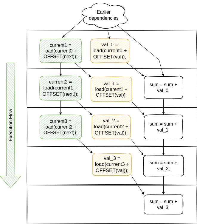
The question is this: can the CPU execute loads independently? If you look at the dependency graph, the answer is no. There is a very hard dependency chain: if a single load in the left column gets stuck (e.g. because of a cache miss), then all the instructions in all subsequent rows are stuck waiting for this load.
In other words, there is a dependency chain of load instructions, where, to process iteration X + 1, the CPU must have finished processing at least the important part of iteration X. In the cases where there is a high data cache miss rate, long load dependency chains can be a disaster for software performance.
Do you need to discuss a performance problem in your project? Or maybe you want a vectorization training for yourself or your team? Contact us
You can also subscribe to our mailing list (link top right of this page) or follow us on LinkedIn , Twitter or Mastodon and get notified as soon as new content becomes available.
What Are the Codes with Low ILP?
Under the assumptions that loads are the critical instructions, we know that codes with loop-carried dependencies where a load in iteration i = X depends on the same or another load from the previous iteration i = X - 1 are codes with low ILP. But, typically, what are those codes? Here are a few examples:
- Operations on linked lists
- Operations on trees
- Operations on hash maps with separate chaining used for collision resolution, in cases where the hash map has many conflicts (because it internally uses a linked list).
The reason for low ILP is quite simple. We cannot move to process the next element in the data structure until we have finished processing the current element.
Techniques Used to Increase Available Instruction-Level Parallelism
In order to add additional ILP to an ILP low memory-bound code, there are two groups of techniques:
- Breaking the dependency chains, where you break the chains by rewriting your datastructure and algorithm.
- Interleaving additional work, where you don’t change your datastructure but process more than one element at a time.
The second technique is more useful because it doesn’t require rewriting the whole datastructure. The first requires more thinking, and by breaking dependency chains you lose some flexibility of pointers.
To my knowledge, there is no extensive list of techniques used to increase available instruction-level parallelism. Here we will present a few ideas on how to increase the available instruction-level parallelism for memory-bound code, but under no circumstances does this list presents all that is possible to do.
Interleaving Additional Work
Consider the task of looking up N values in a tree or a linked list. Instead of traversing the data structure individually, you can traverse the data structure for all N values at once. Here is how it is done.
Linked Lists
When looking up N values in a linked list, instead of traversing the linked list N times, you traverse the linked list only once. While visiting node X, you check if it matches each of N values you want to look up. Then you move to the next node and repeat the process, etc. Here is the code snippet:
current_node = head;

while (current_node) {
    for (int i = 0; i < N; i++) {
        if (values[i] = current_node->value) {
            result[i] = true;
            break;
        }
    }
    current_node = current_node->next;
}
This code might seem less optimal than the original code, but it has a much higher ILP and it is typically much faster. The innermost loop over i can be vectorized as well, which gives it an additional speed boost. We explore this in more detail in the experiments section.
Binary Trees
When looking up N values in a binary tree, instead of performing N individual lookups, we perform lookups for all N values at once. For this we need a temporary array to store the current node for each of the N values. You will need a counter called not_null_count that stores how many values the search hasn’t finished. When the not_null_count becomes 0, the search has finished for all N nodes. Here is the code snippet:
// Initialize the current_nodes to root for
// each of the N values
for (int i = 0; i < N; i++) {
    current_nodes[i] = root;
}

do {
    not_null_count = 0;
    for (int i = 0; i < N; i++) {
        if (current_nodes[i] != nullptr) {
            NodeType* node = current_nodes[i];
            if (values[i] < node->value) {
                current_nodes[i] = node->left;
            } else if (values[i] > node->value) {
                current_nodes[i] = node->right;
            } else {
                current_nodes[i] = nullptr;
                result[i] = true;
            }
            not_null_count++;
        }
    }
} while (not_null_count > 0);
In addition to an increase in instruction-level parallelism, this approach also has a better memory locality. The first few iterations of the do while loops will completely hit the L1 cache, the following few iterations will completely hit the L2 cache, etc. Only the last few iterations will not hit any cache.
For this approach, however, the tree must be balanced. The number of iterations of the do while loop is equal to the tree depth, therefore, with an unbalanced tree, the additional overhead of the inner for loop will probably not pay off.
In the experiment section we measure the effect of interleaving additional work on a binary tree.
A technique of explicit software prefetching combines very nicely with interleaving several dependency chains. We can use explicit software prefetching to prefetch the data we will need for dependency chain X, go do some work on dependency chain Y, and when we return to processing dependency chain X, data needed for X will be already in the fastest level of data cache. Read more about explicit hardware prefetching here.
Do you need to discuss a performance problem in your project? Or maybe you want a vectorization training for yourself or your team? Contact us
You can also subscribe to our mailing list (link top right of this page) or follow us on LinkedIn , Twitter or Mastodon and get notified as soon as new content becomes available.
Breaking Pointer Chains
Another technique to increase ILP is breaking pointer chains. If we somehow manage to break those chains, even partially or conditionally, this can result in a speedup.
Linked Lists
Take for example that we have to lookup N values in a linked list. With N values, we would need to traverse the list N times. But because of the dependency chains, the traversal code will be slow. To break the dependency chain, we traverse the linked list once and create an index: an array of node pointers where a pointer at location X points to the node at location X in the linked list.
In the next step, we don’t iterate the linked list, instead, we iterate the index array. Here is the code snippet that traverses the list:
node* current_node = head;

// Create an index array
while (current_node != nullptr) {
    index_vector.push_back(current_node);
    current_node = current_node->next;
}

// Iterate the index array
for (int i = 0; i < values.size(); i++) {
    for (int j = 0; j < index_vector.size(); j++) {
        if (index_vector[j]->value == values[i]) {
            result[i] = true;
            break;
        }
    }
}
Open Addressing Hash Maps
In software development, two common approaches to collision resolution are separate chaining and open addressing. With separate chaining, when a collision occurs, a linked list of all values belonging to the same bucket is formed. With open addressing, when a collision occurs, the runtime searches the next available buckets in the backing array to store the new value.
When the runtime accesses a collisioned bucket, the performance of open addressing hash map will be faster. There are two reasons for this. The first one is better data locality for the open addressing hash map: there is a high chance that two values corresponding to the same bucket are also in the same cache line. And the second is increased ILP: with open-addressing hash maps, the CPU can issue several parallel loads at once. The reason is same as with linked lists from previous section: the collisioned values form a linked list, and iterating linked list is following a chain of dependencies.
Binary Trees
For binary trees, breaking pointer chains can be done in several ways. One way is to store a binary tree in an array. In this case, the address of the left and right nodes can be calculated by applying a mathematical formula: if the index of the current node in the array is i, then the index of the left node is 2 * i + 1 and the address of the right node is 2 * i + 2. In the experiment section we talk about this.
Binary search in the sorted array is typically faster than a lookup in a binary tree, although the complexity of both lookups is the same O(log n). There are two reasons for this: smaller dataset size (binary trees store only values, no pointers) and increased ILP.
Shortening the Dependency Chain
Making the dependency chain shorter will result in speedup. In the case of a linked list, we can use unrolled linked lists where we store more than one value inside a single linked list node. In the case of trees, replacing binary trees with N-ary trees (e.g. B* trees) shortens the dependency chain (because the tree is shallower).
Both these techniques increase the available ILP: there is more work to be done when processing a single node, and the processing of a single node mostly has good ILP. Also, these techniques increase the locality of reference, which means more data cache hits, less memory traffic, and faster speeds.
Experiments
In this section we will experiment with the various algorithms and ILP. Instruction level parallelism is not possible to measure directly, and also, changing the data layout would result in a different data cache hit rate which would ruin the ILP measurements. Therefore we will take a different approach: we keep the memory layout identical and only change the algorithm.
We measure the runtime, instruction count, and cycles-per-instruction metric (CPI) to get an idea of what is going on. We measure runtime because this is at the end what interests us. We measure instruction count because sometimes the difference in speed can be attributed to a different instruction count and not an improvement in ILP. And finally, CPI metric tells us about hardware efficiency: the smaller the number, the more efficient the algorithm.
All codes are available in our repository.
Interleaving Lookups in a Binary Tree
For the first test of the effect of instruction-level parallelism we use the interleaved binary tree lookup we presented earlier. We use the simple algorithm that works on one-by-one value and we contrast it with the interleaved version. We measure runtimes, instruction count and CPI metric for various binary tree sizes. In both algorithms, the tree’s memory layout remains the same, only the algorithm changes.
We ran the tests on various binary tree sizes. The sizes of binary trees in nodes are: 8K, 16K, 32K, …, 8M, 16M. For each binary tree size we perform 16M lookups in total. This is to get us the feeling about how the runtime is connected to the dataset size.
The first important thing to notice is the instruction count. Interleaved version executes much more instruction than the simple version. For the smallest tree size, it executes 1.8 times more instructions. For the largest tree size, it executes 1.95 times more instructions.
Here are the runtimes of both algorithms depending on the binary tree sizes:
For small tree sizes, there isn’t much of a difference, but the interleaved version is always faster. But as the tree grows, so the relative difference in speed does. When the tree is the largest, the interleaved version is about 2 times faster than the simple version, even though it is executing almost two times as many instructions.
Let’s measure the hardware efficiency. We measure CPI (cycles-per-instruction): the smaller CPI, the better. Here is the graph:
Two things to observe: interleaved version has a much better CPI and CPI grows as the binary tree grows. CPI for the simple version grows very rapidly: from the initial value of 2.72 it grows to 10.6. The growth of the interleaved version is much smaller: from the initial value of 1.27 it grows to 2.77.
I also wanted to plot the peak memory data load rates. The memory subsystem has a peak memory throughput. If our program reaches it, that means that the memory subsystem is the bottleneck and we need to figure out ways how to use it more efficiently. But if the peak is not reached and yet we see that the program is memory-bound, the problem can be because of the low ILP.
Unfortunately, I couldn’t record the data because the hardware counters kept overloading and the data made no sense. What I expected to see was that the interleaved version saturates the memory bus, and the simple version doesn’t. But I couldn’t confirm this.
Do you need to discuss a performance problem in your project? Or maybe you want a vectorization training for yourself or your team? Contact us
You can also subscribe to our mailing list (link top right of this page) or follow us on LinkedIn , Twitter or Mastodon and get notified as soon as new content becomes available.
Breaking Dependencies with Array-Based Binary Tree
For the second test, we store the binary tree in an array. When stored like this we can use arithmetics to calculate the place of the left or the right child. If the node is at position x in the array, its left node is at position 2*x + 1 and its right node is at position 2*x + 2. But, in addition to storing the values, we also store left and right pointers. So, there are two ways to perform lookups in the tree: the first one is using arithmetics, as we just explained, and the second one is following the pointers. The data structure remains the same.
With regards to the number of executed instructions, the array-based version executes 1.42 times more instructions than the pointer-based version for the smallest tree and 1.40 times more instructions for the largest tree.
Here is the graph depicting runtimes for pointer-based and array-based lookup in the identical binary tree:
The runtimes are more or less the same until the tree has 256K nodes. From that point, the pointer-based array becomes much slower. Since a single node has 24 bytes, the total size of the data structure is 6MB. The total size of LLC on the chip we ran test is 6MB, so the performance problems really hit in once the tree doesn’t fit the last level cache anymore.
Let’s look at the hardware efficiency through CPI metric:
Similar to the previous experiment, once the dataset doesn’t fit the LL cache, the CPI gets much worse for the pointer-based binary tree. When the tree is the largest, the efficacy of the pointer-based version is 3.3 times lower than the array-based version.
Do you need to discuss a performance problem in your project? Or maybe you want a vectorization training for yourself or your team? Contact us
You can also subscribe to our mailing list (link top right of this page) or follow us on LinkedIn , Twitter or Mastodon and get notified as soon as new content becomes available.
Breaking Dependencies in a Linked List
For this experiment we use a hybrid linked list: it is a linked list with a maximum capacity, backed by an array. We also introduce a perfect memory ordering: all the nodes that are neighbors in the linked list are also neighbors in memory. Or in other words: addr(next_node) = addr(current_node + 1). We talked about perfect memory ordering our quest for the fastest linked list.
We use several lookup algorithms to lookup values stored in a vector in the linked list. They are:
- Simple: the simplest algorithm takes a value, and iterates the linked list until it finds it or reaches the end of the list. If there are N values to look up, it will iterate the linked list N times.
- Interleaved: interleaved version performs N searches simultaneously. It takes the first node of the list, and performs N comparisons for the first node, then N comparisons for the second node, etc.
- Array: doesn’t iterate the linked list, instead it iterates the underlying array that backs it up. Deleted nodes in the list will have value -1 for the next pointer, so those nodes are skipped.
- Index: it first creates an index array of the linked list as explained in the section Breaking pointer chains. Then it iterates through the index array instead of the linked list.
So, interleaved version would correspond to interleaving additional work and array and index version would correspond to breaking the dependency chain.
The list used for testing has 16M nodes, and we are looking up a total of 128 values. Half of the values do not exist in the linked list, so the lookup algorithm would need to traverse the whole list.
As in the previous examples, we measured runtime, instruction count and CPI for all four types of linked list. We used two linked list memory layouts: the perfect memory layout and a layout where about 25% of the nodes are randomly misplaced. Here are the results:
| Memory layout | Simple | Interleaved | Array | Index |
|---|---|---|---|---|
| Perfect layout | Runtime: 2.74 s Instr: 7817 M CPI: 1.19 | Runtime: 0.69 s Instr: 10855 M CPI: 0.25 | Runtime: 1.79 s Instr: 12507 M CPI: 0.47 | Runtime: 2.16 s Instr: 9515 M CPI: 0.71 |
| Misplaced 25% of the nodes | Runtime: 53.9 s Instr: 7756 M CPI: 13.16 | Runtime: 1.26 s Instr: 10855 M CPI: 0.38 | Runtime: 1.79 s Instr: 12507 CPI: 0.47 | Runtime: 17.11 s Instr: 9442 M CPI: 1.89 |
This table contains a lot of interesting data. Let’s investigate it:
- Perfect layout vs misplaced 25% layout: the change in the data layout has an extreme effect on performance for simple and index versions. The simple version is 19.7 times slower and the index version is 7.9 times slower. This can be completely attributed to data cache misses.
- Simple vs index version: the difference in speed is mostly due to the increase in instruction-level parallelism. Even though the index version executes more instructions, for perfect layout, the index version is 1.27 times faster. For the misplaced layout, the version is 3.15 times faster.
- Array version doesn’t care for memory layout: the reason is that the array version scans the underlying array from left to right in both cases for both versions, so nothing really changes.
- Interleaved version is the fastest: the reason is quite simple. The innermost loop in the interleaved version is a simple
forloop iterating over a vector of integers. From the hardware efficiency point of view, this is very efficient. Those loops also can be vectorized for an additional speed boost, although this didn’t happen in our case.
Conclusion
This post has been very exciting for me to write, because it throws a different light on hardware and how instruction-level parallelism can help us write faster programs.
The crucial note here is memory load dependency: in the presence of high data cache miss rates, memory load dependency can really cripple the software performance. Knowing when load dependencies happen and how to break the dependency chain can help you write much faster software.
With regards to which technique to use, to me, it seems that interleaving additional work is both simpler and more effective than breaking dependency chains. Breaking dependency chains requires a rewrite of both the data structure and the algorithm. Breaking dependency chains is also more difficult to achieve, because those techniques bring come with limitations that make them difficult to use (e.g. inserting a value in an array represented binary tree is not simple, also, not every linked list can be represented as an array).
When there is a load dependency chain but a good memory layout (e.g. perfect memory layout with linked lists), then the benefits of increased ILP are limited.
Do you need to discuss a performance problem in your project? Or maybe you want a vectorization training for yourself or your team? Contact us
You can also subscribe to our mailing list (link top right of this page) or follow us on LinkedIn , Twitter or Mastodon and get notified as soon as new content becomes available.
- Cross-iteration dependency chain is a dependency chain where the instructions in the current iteration depend on the results from instructions in the previous iteration. [↩]
- There is a tool called llvm-mca that you can use to perform dependency analysis, but it works only on assembly code [↩]
- Please note that instructions
if (...) goto ..are not hard dependencies due to speculation, at least when they are speculated correctly (which is the case here). [↩]